


How to Find the Average in Excel?
Are you looking for an easy way to quickly find the average of a set of numbers in Excel? If so, you’ve come to the right place. In this article, we will discuss how to calculate the average of a set of numbers in Excel, and provide a few useful tips to help make the process as efficient and straightforward as possible. Whether you’re a beginner or an experienced Excel user, you’ll be able to find the average of a set of numbers in no time. Let’s get started!
Finding the average in Excel is easy! Here’s how to do it:
- Open the Excel spreadsheet that contains the data you want to use for finding the average.
- Highlight the cells containing the data.
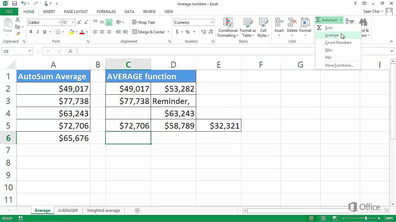
- Click the “Home” tab on the top toolbar.
- Click the “AutoSum” button in the Editing section of the Home tab.
- Press “Enter” or click the “Check Mark” icon to complete the formula.
The average will now be displayed in the cell you selected. If you want to change the average to another cell, click the cell to move the formula.
How to Calculate the Average in Excel?
The average, or mean, of a set of data is a measure of the central tendency of the data set. Excel provides a variety of functions to enable you to calculate the average of a set of data points. This tutorial will show you how to calculate the average using three different methods in Microsoft Excel.
Using the AVERAGE Function
The AVERAGE function is the simplest and most commonly used function to calculate the average. To use the function, enter the range of cells that contains the data points into the parentheses of the function. For example, if the data points are in the range B2:B7, then enter AVERAGE(B2:B7). The result of the function will appear in the cell in which you entered the function.
You can also use the AVERAGE function to calculate the average of a specific set of values. For example, if you want to calculate the average of the numbers 5, 8, and 10, then enter AVERAGE(5,8,10) into a cell. The result of the function will appear in the cell in which you entered the function.
Using the AVERAGEIF Function
The AVERAGEIF function is used to calculate the average of a set of data points based on a specific criterion. For example, if you want to calculate the average of all the numbers in the range B2:B7 that are greater than 5, then you would enter AVERAGEIF(B2:B7,”>5″). The result of the function will appear in the cell in which you entered the function.
You can also use the AVERAGEIF function to calculate the average of a specific set of values. For example, if you want to calculate the average of the numbers 5, 8, and 10 that are greater than 5, then enter AVERAGEIF(5,8,10,”>5″) into a cell. The result of the function will appear in the cell in which you entered the function.
Using the AVERAGEIFS Function
The AVERAGEIFS function is used to calculate the average of a set of data points based on multiple criteria. For example, if you want to calculate the average of all the numbers in the range B2:B7 that are greater than 5 and less than 10, then you would enter AVERAGEIFS(B2:B7,”>5″,”5″,”Frequently Asked Questions
Q1. How do I find the average of a range of cells in Excel?
A1. To find the average of a range of cells in Excel, you can use the AVERAGE function. The syntax for this function is “=AVERAGE(number1, number2,…)” where number1, number2, etc. are the cells you want to average. You can also use the range selector to select a range of cells, and the AVERAGE function will automatically calculate the average of all the cells in the range. For example, if your range of cells is A1:A10, the syntax for the AVERAGE function would be “=AVERAGE(A1:A10)”.
Q2. How do I find the average of a column in Excel?
A2. To find the average of a column in Excel, you can use the AVERAGE function with the range selector. For example, if the column you want to find the average of is column A, the syntax for the AVERAGE function would be “=AVERAGE(A:A)”. This will automatically calculate the average of all the cells in the column.
Q3. How do I find the average of a row in Excel?
A3. To find the average of a row in Excel, you can use the AVERAGE function with the range selector. For example, if the row you want to find the average of is row 1, the syntax for the AVERAGE function would be “=AVERAGE(1:1)”. This will automatically calculate the average of all the cells in the row.
Q4. How do I find the average of multiple columns in Excel?
A4. To find the average of multiple columns in Excel, you can use the AVERAGE function with the range selector. For example, if the columns you want to find the average of are columns A and B, the syntax for the AVERAGE function would be “=AVERAGE(A:B)”. This will automatically calculate the average of all the cells in the columns.
Q5. How do I find the average of multiple rows in Excel?
A5. To find the average of multiple rows in Excel, you can use the AVERAGE function with the range selector. For example, if the rows you want to find the average of are rows 1 and 2, the syntax for the AVERAGE function would be “=AVERAGE(1:2)”. This will automatically calculate the average of all the cells in the rows.
Q6. How do I find the average excluding certain cells in Excel?
A6. To find the average excluding certain cells in Excel, you can use the AVERAGE function with the range selector and the IF function. The syntax for the IF function is “=IF(logical_test, value_if_true, value_if_false)”. In this case, the logical_test would be “cell_reference value”, where cell_reference is the cell you want to exclude and value is the value of the cell you want to exclude. The value_if_true would be the cell_reference and the value_if_false would be 0. You can then use the IF function in the AVERAGE function. For example, if the range of cells you want to average is A1:A10 and you want to exclude cell A5, the syntax for the AVERAGE function would be “=AVERAGE(IF(A1:A10A5,A1:A10,0))”. This will calculate the average of all the cells in the range except cell A5.
Using the Excel Average and AverageA functions
Knowing how to find the average in Excel is an important skill to have in today’s world. Understanding how to use the AVERAGE function in Excel can help you make calculations quickly and accurately. This skill is valuable in any profession, as it can help you to save time and make more informed decisions. With this knowledge, you can confidently use the AVERAGE function in Excel and be sure of the results.


