


How to Add Negative Numbers in Excel?

Do you ever find yourself struggling to add negative numbers in Excel? If you said “yes,” then you’ve come to the right place! In this article, we’ll be exploring the various methods for adding negative numbers in Excel, as well as some tips and tricks to make the process easier. So, let’s get started!
Adding negative numbers in Excel is easy. To start, open your spreadsheet, select the cell you want to add the negative numbers to, and enter the numbers you want to add. Then, press the “+” button in the formula bar, which will add the numbers together. If the result of the addition is negative, Excel will display a minus sign in front of the result.
If you need to add more than two numbers together, simply repeat the process by pressing the “+” button for each number you want to add. For example, to add -5, -7, and -9 together, you would press the “+” button once to add -5 and -7 together, then press it again to add the result and -9.
To subtract negative numbers, you can use the same process. Select the cell you want to subtract the numbers from, enter the numbers you want to subtract, and press the “-” button in the formula bar. Excel will subtract the numbers and display the result.
Adding Negative Numbers in Microsoft Excel
Microsoft Excel is a powerful spreadsheet application that is used for a variety of calculations and data analysis. Excel allows users to perform basic mathematical operations such as addition, subtraction, multiplication, and division. In addition, Excel also allows users to add negative numbers. Adding negative numbers in Excel can be done in a few simple steps.
Step 1: Entering the Data
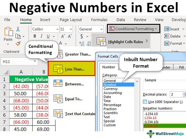
The first step to adding negative numbers in Excel is to enter the data. To do this, open the Excel file and select the cells that you want to add. Once the cells are selected, type in the negative numbers that you want to add. Once you have entered the data, it is important to make sure that the cells are formatted correctly. To format the cells, right-click on the cell and select the “Format Cells” option. This will open a dialog box that will allow you to set the cell type, alignment, and other formatting options.
Step 2: Adding the Numbers
The second step to adding negative numbers in Excel is to add the numbers. To do this, select the cell that will contain the sum of the negative numbers and type in the formula “=SUM(A1:A5)”. This will add the numbers in the cells A1, A2, A3, A4, and A5. If you want to add a range of cells, you can use the formula “=SUM(A1:A10)”.
Step 3: Displaying the Result
The third step to adding negative numbers in Excel is to display the result. To do this, select the cell that contains the sum of the cells and click the “Calculate” button. This will display the result in the selected cell.
Subtracting Negative Numbers in Microsoft Excel
Subtracting negative numbers in Excel is similar to adding them. The first step is to enter the data. This can be done in the same way as adding the numbers. Once the data is entered, select the cell that will contain the result and type in the formula “=SUM(A1:A5)-SUM(A6:A10)”. This will subtract the numbers in the cells A1, A2, A3, A4, and A5 from the numbers in the cells A6, A7, A8, A9, and A10.
Step 1: Entering the Data
The first step to subtracting negative numbers in Excel is to enter the data. To do this, open the Excel file and select the cells that you want to subtract. Once the cells are selected, type in the negative numbers that you want to subtract. Once you have entered the data, it is important to make sure that the cells are formatted correctly. To format the cells, right-click on the cell and select the “Format Cells” option. This will open a dialog box that will allow you to set the cell type, alignment, and other formatting options.
Step 2: Subtracting the Numbers
The second step to subtracting negative numbers in Excel is to subtract the numbers. To do this, select the cell that will contain the difference of the negative numbers and type in the formula “=SUM(A1:A5)-SUM(A6:A10)”. This will subtract the numbers in the cells A1, A2, A3, A4, and A5 from the numbers in the cells A6, A7, A8, A9, and A10.
Multiplying Negative Numbers in Microsoft Excel
Multiplying negative numbers in Excel is similar to adding or subtracting them. The first step is to enter the data. This can be done in the same way as adding or subtracting the numbers. Once the data is entered, select the cell that will contain the result and type in the formula “=PRODUCT(A1:A5)”. This will multiply the numbers in the cells A1, A2, A3, A4, and A5.
Step 1: Entering the Data
The first step to multiplying negative numbers in Excel is to enter the data. To do this, open the Excel file and select the cells that you want to multiply. Once the cells are selected, type in the negative numbers that you want to multiply. Once you have entered the data, it is important to make sure that the cells are formatted correctly. To format the cells, right-click on the cell and select the “Format Cells” option. This will open a dialog box that will allow you to set the cell type, alignment, and other formatting options.
Step 2: Multiplying the Numbers
The second step to multiplying negative numbers in Excel is to multiply the numbers. To do this, select the cell that will contain the product of the negative numbers and type in the formula “=PRODUCT(A1:A5)”. This will multiply the numbers in the cells A1, A2, A3, A4, and A5.
Dividing Negative Numbers in Microsoft Excel
Dividing negative numbers in Excel is similar to adding, subtracting, or multiplying them. The first step is to enter the data. This can be done in the same way as adding, subtracting, or multiplying the numbers. Once the data is entered, select the cell that will contain the result and type in the formula “=DIVIDE(A1:A5)”. This will divide the numbers in the cells A1, A2, A3, A4, and A5.
Step 1: Entering the Data
The first step to dividing negative numbers in Excel is to enter the data. To do this, open the Excel file and select the cells that you want to divide. Once the cells are selected, type in the negative numbers that you want to divide. Once you have entered the data, it is important to make sure that the cells are formatted correctly. To format the cells, right-click on the cell and select the “Format Cells” option. This will open a dialog box that will allow you to set the cell type, alignment, and other formatting options.
Step 2: Dividing the Numbers
The second step to dividing negative numbers in Excel is to divide the numbers. To do this, select the cell that will contain the quotient of the negative numbers and type in the formula “=DIVIDE(A1:A5)”. This will divide the numbers in the cells A1, A2, A3, A4, and A5.
Frequently Asked Questions
What is the Formula to Add Negative Numbers in Excel?
The formula to add negative numbers in Excel is =SUM(number1, number2, …). This formula will add all the cells or ranges of cells that are provided as arguments.
How Do I Enter Negative Numbers in Excel?
Negative numbers can be entered in Excel by simply typing the negative sign before the number, such as -20. Alternatively, the number can be preceded by an equals sign, such as =-20, or enclosed in parentheses, such as (-20).
How Do I Add Multiple Negative Numbers in Excel?
To add multiple negative numbers in Excel, you can use the =SUM(number1, number2, …) formula. This formula will take all the cells or ranges of cells that are provided as arguments and add them together.
How Do I Automatically Subtract Negative Numbers in Excel?
To automatically subtract negative numbers in Excel, you can use the =SUM(number1, -number2, …) formula. This is the same formula as the one used to add negative numbers, but with a negative sign before the number to be subtracted.
How Do I Find the Sum of Positive and Negative Numbers in Excel?
To find the sum of both positive and negative numbers in Excel, you can use the =SUM(number1, number2, …) formula. This formula will take all the cells or ranges of cells that are provided as arguments and add them together, including both positive and negative numbers.
What Does the Formula =SUM(number1, number2, …) Calculate?
The formula =SUM(number1, number2, …) calculates the sum of all the cells or ranges of cells that are provided as arguments. This formula can be used to add both positive and negative numbers in Excel.
Sum Positive and Negative Numbers with the SIGN (and SUMIF) Function
Adding negative numbers in Excel can be a tricky task, but with a few helpful tips, you can quickly become an Excel expert. With some basic knowledge of the formula and calculation methods, you can easily add and subtract negative numbers in Excel. From quickly adding large sets of data to creating more complex formulas, understanding how to add and subtract negative numbers in Excel can help you become a more efficient and successful user of the popular spreadsheet application.


