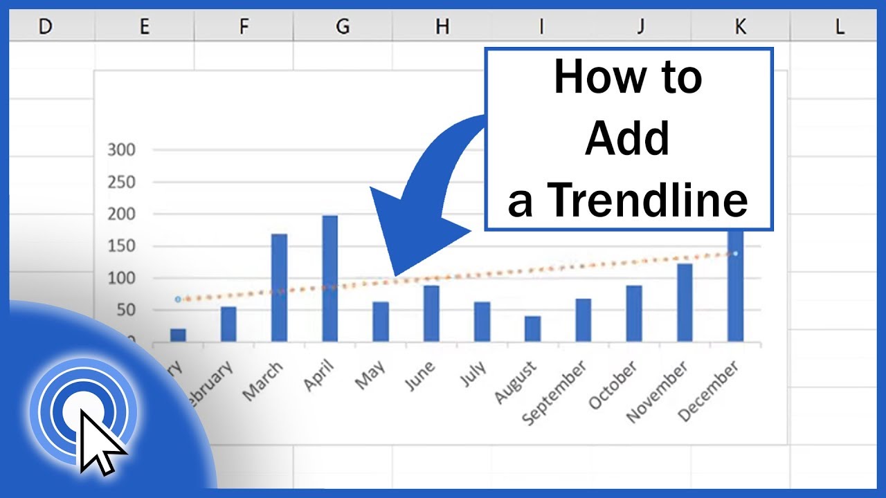
How to Make a Trendline in Excel?

Do you need to create a trendline in Excel to make sense of your data? Making a trendline in Excel can be a great way to visualize the relationship between different data points and get a better understanding of your data. In this article, we will provide step-by-step instructions on how to make a trendline in Excel, so you can make the most of your data.

Making a Trendline in Excel

A trendline is a great way to display the data in a graph or chart. It can be used to make predictions about future trends and to track the progress of a project over time. Excel makes it easy to create a trendline, though the exact steps may vary slightly depending on your version of Excel. This article will outline the basic steps for creating a trendline in Excel.

Step 1: Open the Chart or Graph

The first step is to open the chart or graph that you wish to add a trendline to. If you have already created a chart or graph in Excel, simply open the file and select the chart or graph. If you need to create a chart or graph, open a new Excel file and select the type of chart or graph you wish to create.

Step 2: Add Data to the Chart or Graph

Once you have opened the chart or graph, add the data points you want to include. To do this, select the blank graph and click the “Data” tab. A window will appear where you can enter your data. Once you have entered the data, click “OK” to close the window. Your data points should now appear on the chart or graph.

Step 3: Select the Trendline Option

Now that you have added the data points to your chart or graph, it is time to add the trendline. To do this, select the chart or graph and click the “Chart Tools” tab. Under this tab, select the “Layout” option. A menu will appear with several options, including “Trendline”. Select this option and a dialogue box will appear.

Step 4: Choose the Type of Trendline

In the dialogue box, you will be given the option to choose the type of trendline you wish to use. The types of trendlines available are Linear, Exponential, Polynomial, and Logarithmic. Select the type of trendline you wish to use and click “OK”.

Step 5: Adjust the Trendline Settings

The next step is to adjust the settings for your trendline. In the dialogue box, you will be given the option to adjust the intercept, the order, and the period. The intercept is the point at which the trendline crosses the y-axis. The order is the order of the polynomial equation used to calculate the trendline. The period is the number of data points used in the trendline calculation. Once you have adjusted the settings, click “OK”.

Step 6: View the Trendline

Your trendline should now appear on the chart or graph. You can adjust the settings if needed and view the trendline in the graph. You can also add additional data points to the chart or graph and the trendline will adjust accordingly.

Few Frequently Asked Questions

How do I create a trendline in Excel?

To create a trendline in Excel, first select the data you want to plot. Then, open the Insert tab and click on the line chart icon. In the resulting chart, right-click on the data series and select Add Trendline. A window will appear with a variety of options for customizing the trendline. You can change the type of trendline, set intercepts and display equation and R-squared values. Once you have configured the options, click OK to apply the trendline to your chart.

What types of trendlines can be created in Excel?

Excel offers several types of trendlines that can be used to visualize data. The most commonly used type is linear, which plots a straight line through the data points. Other types of trendlines include exponential, logarithmic, polynomial, and power. Each type of trendline is best suited for different types of data. Experimenting with different types can help you determine which one is most appropriate for your data.

How do I display the equation and R-squared value of a trendline?

To display the equation and R-squared value of a trendline, first add the trendline to your chart. Then, right-click on the trendline and select Format Trendline. In the resulting window, check the boxes for Display Equation on Chart and Display R-Squared Value on Chart. Click OK to apply the changes and the equation and R-squared value will be displayed on your chart.

Can I change the intercepts of a trendline in Excel?

Yes, it is possible to change the intercepts of a trendline in Excel. To do this, first add the trendline to your chart. Then, right-click on the trendline and select Format Trendline. In the resulting window, select the Options tab and check the box for Set Intercept. You can then enter the desired intercepts for the trendline and click OK to apply the changes.

Can I add more than one trendline to a chart in Excel?

Yes, it is possible to add more than one trendline to a chart in Excel. To do this, first add the first trendline to your chart. Then, right-click on the data series and select Add Trendline. In the resulting window, select a different type of trendline and click OK to apply the changes. Repeat this process for each trendline you wish to add.

How do I remove a trendline from a chart in Excel?

To remove a trendline from a chart in Excel, first select the chart. Then, right-click on the trendline and select Delete. The trendline will be removed from the chart. You can also select the trendline and press the Delete key on your keyboard to remove it.

How to Add a Trendline in Excel

Creating a trendline in Excel is easy and can be done in just a few steps. By understanding how to make a trendline in Excel and the various different options available, you can create powerful visuals to better understand the data in your spreadsheet and make more informed decisions. In conclusion, the trendline feature in Excel is an invaluable tool for visually analyzing your data, and can help you make more informed decisions quickly and easily.