


How to Use Hlookup Function in Excel?

If you are an Excel user, then you know how important it is to know how to use the Hlookup function. The Hlookup function is a powerful tool that can help you quickly look up and compare data in spreadsheets. It can be used to compare data between two or more columns and find specific information. In this article, we will explore how to use the Hlookup function in Excel. We will look at how to set up the function and how to use it to find and compare data. So, if you want to become an Excel power user, read on to learn how to use the Hlookup function in Excel.
- Open a spreadsheet with data.
- Identify the cell containing the value you want to search for.
- Identify the range in which the value you want to search for is located.
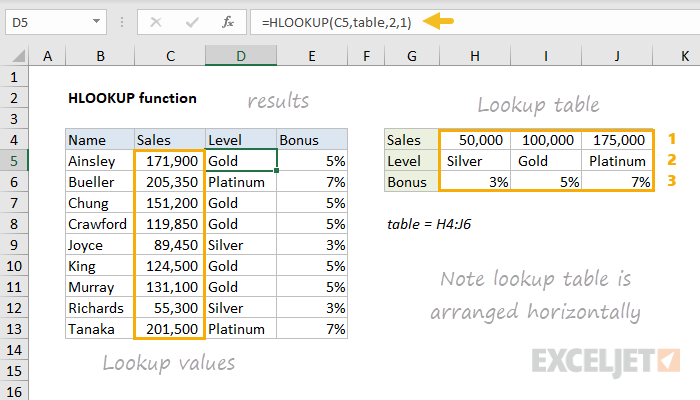
- Enter the ‘HLOOKUP’ function into a cell: =HLOOKUP(cell, range, column_num, exact_match).
- Check the results.
What is the Hlookup Function in Excel?
The Hlookup function in Microsoft Excel is a powerful tool for searching for data in a large spreadsheet. It is a function that searches for a specific value in the top row of a table array and then returns a value from the same column in the same row. This makes it easy to look up data quickly without having to scroll through the entire spreadsheet. Hlookup can be used to quickly find information in data tables, such as employee names, salary information, or other types of data.
In addition to being a quick way to look up data, Hlookup can also be used to compare data between different tables. This can be especially useful when analyzing data from multiple sources. For example, if a company wanted to compare sales figures from different stores, they could use Hlookup to quickly compare the data from each store and make decisions based on the results.
How to Use Hlookup Function in Excel?
Using the Hlookup function in Excel is simple. To use it, open the spreadsheet with the data you want to look up and select the cell where you want the result to appear. Then, enter the Hlookup formula, including the table array, the value you want to look up, the row number, and the column number.
For example, if you wanted to look up the name of an employee whose ID number is 1234, you would enter the following formula: =HLOOKUP(1234, A1:E5, 2, FALSE). This formula would search the table array from A1 to E5 for the number 1234, and if it is found, it would return the value from the second column in the same row.
Required Arguments
The Hlookup function requires four arguments. The first is the value you are looking for, which can be a number, text, or a cell reference. The second is the table array, which is the range of cells that contains the data you are looking for. The third is the row number, which is the row in the table array that contains the value you are looking for. Finally, the fourth argument is whether the lookup is an exact match or not.
Optional Arguments
The Hlookup function also has two optional arguments. The first is the column number, which is the column in the table array that contains the value you are looking for. The second is the range lookup, which is whether you want an exact match or an approximate match.
Using Hlookup with Other Functions
Hlookup can be used in combination with other functions in Excel to perform more complex calculations. For example, the VLOOKUP function can be used in combination with Hlookup to return data from different tables. This can be useful when comparing data from multiple sources.
Using Hlookup for Conditional Formatting
The Hlookup function can also be used in conjunction with conditional formatting in Excel. This can be useful when you want to highlight data based on certain criteria. For example, you may want to highlight data that falls within a certain range or that meets certain criteria.
Using Hlookup to Automate Tasks
The Hlookup function can also be used to automate tasks in Excel. For example, you can use it to create formulas that will automatically update when data changes. This can be useful for quickly and accurately updating data that is constantly changing.
Using Hlookup to Create Custom Dashboards
The Hlookup function can also be used to create custom dashboards in Excel. This can be useful for quickly visualizing data in an easy-to-read format. You can use the Hlookup function to quickly create charts and graphs that can help you analyze data and make decisions.
Related Faq
What is the Hlookup Function?
The Hlookup function in Excel is a function used to search for a specific value in the top row of a table and return the corresponding value from another row in the same table. It is similar to the Vlookup function, however, the Hlookup searches for the value in the first row of the table instead of the first column. It is a useful tool for finding data quickly in large tables.
How is the Hlookup Function Used?
The Hlookup function is used to search for a value in the top row of a table and return a corresponding value from another row in the same table. The syntax for the Hlookup function is “Hlookup (lookup_value, table_array, row_index_num,
What are the Benefits of Using the Hlookup Function?
One of the main benefits of using the Hlookup function is that it can search for values quickly and accurately. With large tables, it is often difficult to manually look for a specific value. The Hlookup function makes this process much easier and more efficient. Additionally, the Hlookup function can be used to compare data from different rows in the same table. This can be useful for making comparisons between different types of data.
What are the Limitations of the Hlookup Function?
One of the main limitations of the Hlookup function is that it can only search for values in the top row of the table. This means that if the value you are searching for is not in the top row, you will not be able to use the Hlookup function to find it. Additionally, the Hlookup function can only return values from the same row as the value you are searching for. This means that if you need to return a value from a different row, you will need to use a different function.
How Can You Troubleshoot an Hlookup Function?
If you are having difficulty getting the Hlookup function to work correctly, the first thing you should do is check the syntax of the function to make sure it is correct. Additionally, you should double-check the range of cells that you are searching, as well as the row index number. If the function is still not returning the expected result, you may need to check to make sure the value you are searching for is actually in the top row of the table and that the row index number is correct.
What are Some Alternatives to the Hlookup Function?
If the Hlookup function is not suitable for your needs, there are a few other functions that you can use to search for data in Excel. The Vlookup function is similar to the Hlookup function, except that it searches for values in the first column of the table. Additionally, you can use the Index and Match functions to search for values in a table. The Index function can be used to return a value from any row or column in a table, while the Match function can be used to find a specific value in a table.
How to use the HLOOKUP function in Excel
The HLOOKUP function in Excel is a useful tool to help you quickly find data in a worksheet. It can save you time and effort when working with large sheets of data and can be used to cross-reference information from different sheets. With just a few simple steps, you can easily use the HLOOKUP function to help you find the data you need in no time.


