


How to Match 2 Columns in Excel?

Are you looking for an easy way to quickly match data in two columns in Excel? We’ve got you covered! In this guide, we will cover the steps for matching two columns in Excel and provide tips for how to make the process as fast and efficient as possible. By the time you’re done, you’ll have the confidence to quickly and accurately match columns in Excel. Let’s get started!
Choose which column you want to compare and then click on “OK”. Excel will now highlight any cells that have the same value in both columns. To ensure accuracy, you can also select “Case Sensitive” or “Exact Match” options.
You can also use the “VLOOKUP” function to match two columns. This allows you to look up values in one column and return a value from another column. To do this, select the “Formulas” tab and enter the VLOOKUP formula. You will need to enter the range of cells, the column you wish to search, and the column from which you want to return the value.
Matching Data in 2 Excel Columns
Excel is a very powerful tool for analyzing and manipulating data. It can help you quickly match data in two columns, allowing you to identify the records that are the same and those that are different. In this tutorial, we will show you how to match two columns in Excel.
The first step is to make sure that the columns you want to compare are both in the same format. This means that they should have the same data type, such as numbers, text, or dates. If they are not in the same format, you will need to convert them before you can match them.
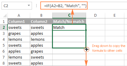
The next step is to select the cells you want to compare. To do this, click on the first cell in the first column and drag your mouse to the last cell in the second column. This will select the range of cells that you want to compare.
Using the VLOOKUP Function
One of the easiest ways to match two columns in Excel is to use the VLOOKUP function. This function takes two arguments, the first being the value you want to search for and the second being the range of cells that you want to search. It then returns the row number of the first cell in the range that matches the value.
For example, if you have a list of names in column A and a list of ages in column B, you can use the VLOOKUP function to find the age of a particular name. To do this, you would enter the name in the first argument and the range of cells in column B in the second argument. The VLOOKUP function will then return the age of the name in column B.
Using the MATCH Function
The MATCH function is another useful way to match two columns in Excel. This function takes two arguments, the first being the value you want to search for and the second being the range of cells that you want to search. It then returns the position of the first cell in the range that matches the value.
For example, if you have a list of names in column A and a list of ages in column B, you can use the MATCH function to find the position of a particular name. To do this, you would enter the name in the first argument and the range of cells in column A in the second argument. The MATCH function will then return the position of the name in column A.
Using the INDEX and MATCH Functions Together
The INDEX and MATCH functions can be used together to match two columns in Excel. The INDEX function takes two arguments, the first being the range of cells that you want to search and the second being the position of the cell you want to return. The MATCH function takes two arguments, the first being the value you want to search for and the second being the range of cells that you want to search.
For example, if you have a list of names in column A and a list of ages in column B, you can use the INDEX and MATCH functions together to find the age of a particular name. To do this, you would enter the range of cells in column B in the first argument of the INDEX function and the range of cells in column A in the first argument of the MATCH function. The MATCH function will then return the position of the name in column A and the INDEX function will return the age of the name in column B.
Using Conditional Formatting
Another way to match two columns in Excel is to use conditional formatting. This is a feature that allows you to highlight certain cells based on certain criteria. To do this, you would select the range of cells you want to compare and then select the “Conditional Formatting” option from the Home tab.
You can then select the “Highlight Cells Rules” option and choose the “Duplicate Values” option. This will highlight any cells in the range that have the same value. This can be a useful way to quickly find any data that is the same in two columns.
Using the FILTER Function
The FILTER function is another useful way to match two columns in Excel. This function takes two arguments, the first being the range of cells you want to search and the second being the value you want to search for. It then returns the rows that contain the value.
For example, if you have a list of names in column A and a list of ages in column B, you can use the FILTER function to find the rows that contain a particular name. To do this, you would enter the range of cells in column A in the first argument and the name in the second argument. The FILTER function will then return the rows that contain the name.
Using the COUNTIF Function
The COUNTIF function is another useful way to match two columns in Excel. This function takes two arguments, the first being the range of cells you want to search and the second being the value you want to count. It then returns the number of cells in the range that contain the value.
For example, if you have a list of names in column A and a list of ages in column B, you can use the COUNTIF function to find the number of names that are the same. To do this, you would enter the range of cells in column A in the first argument and the range of cells in column B in the second argument. The COUNTIF function will then return the number of names that are the same.
Related Faq
What is the purpose of matching two columns in Excel?
The purpose of matching two columns in Excel is to compare two lists of data and find any matches between them. This is a useful tool for data analysis and can help you identify trends, find discrepancies, and spot errors in the data. For example, you may want to compare two customer lists to find any duplicate customers or you may want to compare two lists of sales figures to identify any potential sales trends. Matching two columns in Excel can also help you identify any potential problems with your data, such as missing or incorrect data.
What are the steps to match two columns in Excel?
The steps to match two columns in Excel are as follows:
1. Open the Excel file containing the two columns you would like to match.
2. Select the two columns to match.
3. Click the “Data” tab in the ribbon bar and select “Sort & Filter”.
4. Select “Filter” and click the dropdown arrow in the heading of each column to be matched.
5. Select “Sort A to Z” or “Sort Z to A” in the dropdown menu for each column.
6. Select the “Match” button in the “Sort & Filter” menu.
7. The matched values will be highlighted in the two columns.
What options are available for matching two columns in Excel?
When matching two columns in Excel, you have the option to match the entire row or only a single column in the row. You can also choose to match only the values that are exactly the same, or you can choose to match any value that is similar. Additionally, you can choose to match only the values that are within a certain range, or you can choose to match any value that is close in value to the original.
What are the benefits of matching two columns in Excel?
Matching two columns in Excel can be a useful tool for data analysis. By identifying any matches between two columns, you can quickly and easily spot errors in your data or identify any trends or discrepancies. You can also use the matched values to quickly update your data or to compare values between different datasets.
Are there any risks associated with matching two columns in Excel?
Yes, there are some risks associated with matching two columns in Excel. For example, if you are matching two columns with similar values, it is possible that you could mistakenly match values that are not actually the same. Additionally, if you are matching two columns with numerical values, it is possible that you could mistakenly match values that are within a certain range, but not actually the same.
What are some tips for matching two columns in Excel?
When matching two columns in Excel, it is important to make sure that the data is accurate and up to date. Additionally, it is important to double-check the matched values to make sure that they are actually the same. Lastly, it is important to know the range of values that you are looking for and to use the appropriate filtering options to ensure that you are only matching the correct values.
How to Use Excel to Match Up Two Different Columns : Using Excel & Spreadsheets
Matching two columns in Excel is a simple task that can be completed quickly and easily. With just a few clicks, you can create a new column that matches two columns for further calculations and analysis. Knowing how to match two columns in Excel can be a powerful tool for anyone who needs to compare and analyze data. So take the time to learn the process and unlock the power of Excel for your data needs.


